library(reactable)
library(reactablefmtr)
library(tidyverse)
Data visualisation is a key aspect of communicating our story or message behind the data we have. While it is common to visualise data using a myriad of graphs, tables may be more appropriate or effective at times to present numerous data information. In addition, such mode of data visualisation can be even more effective by allowing readers to interact with the table. This blog post documents my attempt to visualise data on the FIFA World Cup 22 participating teams with interactive tables using R programming language.
Required Libraries
There are plenty of different packages available in R to create interactive tables. In this blog post, the {reactable} package was used to first build the interactive table and the {reactablefmtr} package was utilised for styling purpose. Besides that, {tidyverse} was used mainly to help with data wrangling.
Data
This post used a total of three datasets to show information of all FIFA World Cup 22’s participating teams’ historical appearances in the knockout stages of previous editions of the competition:
Results of all World Cup matches played in history (Source: Kaggle)
Participating teams in FIFA World Cup 22 and their respective FIFA rankings and points
Country flag dataset with URL addresses of country flag images
wc_matches <- read.csv("wcmatches.csv")
wc22_teams <- read.csv("wc22teams.csv")
country_flags<-read.csv("country_flags_dataset.csv")
Data Wrangling
First, data wrangling was performed to retrieve and summarise the required data for visualisation. These data were then joined together as a dataframe for building the interactive table. You may see the full code for data wrangling by unfolding the code chunk below under the code tab. Also, you may see a description of the final dataframe variables under the data tab.
Code
# Modify dataframe into long format to see all participating teams in one column
wc_matches_v2 <- wc_matches%>%
  pivot_longer(cols = c(home_team, away_team),
               names_to = "Home_away",values_to = "Team")

# Some countries require renaming
wc_matches_v2[(wc_matches_v2$Team == "West Germany"), c("Team")] <- "Germany"
wc_matches_v2[(!is.na(wc_matches_v2$winning_team) & wc_matches_v2$winning_team == "West Germany"), c("winning_team")] <- "Germany"

# Summarising counts for each country's appearance in different stages of the competition

# Round of 16s
df_round16 <- wc_matches_v2|>
  filter(stage == "Round of 16")|>
  group_by(Team)|>
  count() |>
  rename("Round_16" = "n")
# Quarter-finals
df_quarter <- wc_matches_v2|>
  filter(stage == "Quarterfinals")|>
  group_by(Team)|>
  count()|>
  rename("Quarter_finals" = "n")
# Semi-finals
df_semi <- wc_matches_v2|>
  filter(stage == "Semifinals")|>
  group_by(Team)|>
  count()|>
  rename("Semi_finals" = "n")
# Finals
df_final <- wc_matches_v2|>
  filter(stage == "Final")|>
  group_by(Team)|>
  count()|>
  rename("Finals" = "n")
# World cup wins
df_wc_wins <- wc_matches_v2|>
  filter(stage == "Final")|>
  group_by(winning_team)|>
  count()|>
  mutate(n = n/2)

# The finals of 1950 competition was played in a round robin format instead and Uruguay was the winner thus adding one count for Uruguay
df_wc_wins_v2<-df_wc_wins|>
  mutate(n = ifelse(winning_team == "Uruguay", n+1, n))|>
  rename("Wins" = "n",
         "Team" = "winning_team")

# Join all dataframes
merged_results_df<-df_round16|>
  left_join(df_quarter)|>
  left_join(df_semi)|>
  left_join(df_final)|>
  left_join(df_wc_wins_v2)|>
  replace_na(list("Quarter_finals" = 0,
                  "Semi_finals" = 0,
                  "Finals" = 0,
                  "Wins" = 0))

# Processing of flag data for joining
country_flags_v2 <- country_flags|>
  rename("Team" = "Country")

# Join the data for teams participating in the Fifa world cup 22
# First filter the teams that are participating in the Fifa world cup 22
filtered_df<-merged_results_df|>
  semi_join(wc22_teams, by = "Team")
# Finally, use left join to merge with the world cup 22 team dataset
working_data <- wc22_teams|>
  left_join(filtered_df)|>
  left_join(country_flags_v2)|>
  replace_na(list("Round_16" = 0,
                  "Quarter_finals" = 0,
                  "Semi_finals" = 0,
                  "Finals" = 0,
                  "Wins" = 0))|>
  select("ImageURL", "Team", "Fifa_rank", "Ranking_points",
         "Round_16","Quarter_finals","Semi_finals",
         "Finals", "Wins")|>
  mutate(Ranking_points = round(Ranking_points, 2))
Rows: 32
Columns: 9
$ ImageURL <chr> "https://upload.wikimedia.org/wikipedia/commons/1/1a/Fl…
$ Team <chr> "Argentina", "Australia", "Belgium", "Brazil", "Cameroo…
$ Fifa_rank <int> 3, 38, 2, 1, 43, 41, 31, 12, 10, 44, 5, 4, 11, 61, 20, …
$ Ranking_points <dbl> 1773.88, 1488.72, 1816.71, 1841.30, 1471.44, 1475.00, 1…
$ Round_16 <int> 9, 1, 8, 11, 1, 0, 2, 2, 4, 1, 7, 7, 11, 2, 0, 3, 8, 1,…
$ Quarter_finals <int> 7, 0, 3, 14, 1, 0, 1, 2, 1, 0, 9, 7, 14, 1, 0, 0, 2, 0,…
$ Semi_finals <int> 4, 0, 2, 8, 0, 0, 0, 2, 0, 0, 3, 6, 12, 0, 0, 0, 0, 0, …
$ Finals <int> 5, 0, 0, 6, 0, 0, 0, 1, 0, 0, 1, 3, 8, 0, 0, 0, 0, 0, 3…
$ Wins <dbl> 2, 0, 0, 5, 0, 0, 0, 0, 0, 0, 1, 2, 4, 0, 0, 0, 0, 0, 0…Creating Interactive Table
Next, turning our dataframe into a table can be simply executed by passing the name of the dataframe as a single argument in the reactable() function. By default, the table would be paginated with ten rows of data per page. The page size could be altered by specifying the defaultPageSize argument.
Importantly, the table is not static and readers can interact with it. For example, you may sort the data by each column by clicking on the column’s header.
# Removing the ImageURL column from the dataframe for ease of preview

working_data_v2 <- working_data|>
  select(-ImageURL)

reactable(working_data_v2,
          # Default page size is 10 rows per page
          defaultPageSize = 5)
As seen above,the table headers correspond to the variable names in the dataframe by default. We may specify the names for each column under the colDef function. In addition, various arguments (e.g., cell alignment, style) can be passed through this function to customise the columns.
reactable(working_data_v2,
          # Sorting our table based on the FIFA ranking by default
          defaultSorted = "Fifa_rank",
          # Defining vertical and horizontal alignment of each column cell to be center by default
          defaultColDef = colDef(
            vAlign = "center",
            align = "center"
          ),
          columns = list(
          Team = colDef(name = "Team",
                          width = 105),
          Fifa_rank = colDef(name = "FIFA Ranking"),
          Ranking_points = colDef(name = "FIFA Ranking Points"),
          Round_16 = colDef(name = "Round of 16"),
          Quarter_finals = colDef(name = "Quarter-Final"),
          Semi_finals = colDef(name = "Semi-Final"),
          Finals = colDef(name = "Final"),
          Wins = colDef(name = "Champion")
          ))
Beautify our Table
Once we are satisfied with how the data information are presented, it is time to turn our focus to the aesthetics to make our table more attractive.
Insert images
The {reactablefmtr} package provides several additional functions to enhance the styling and formatting of tables built with the {reactable} package. Specifically, the embed_img() function, as the name suggests, enables us to embed images directly from the web into the table. In this blog post, I embedded country flag images into the table with the URL addresses from the country flags dataset.
reactable(working_data,
          # Sorting our table based on the FIFA ranking by default
          defaultSorted = "Fifa_rank",
          # Defining vertical and horizontal alignment of each column cell to be center by default
          defaultColDef = colDef(
            vAlign = "center",
            align = "center"
          ),
          columns = list(
          # Embedding country flag images into the first column. You may specify the height and width of the cell.
        ImageURL = colDef(cell = embed_img(working_data,width = 45, height = 40,
                                        horizontal_align = "center"), name = ""),
          Team = colDef(name = "Team",
                          width = 115),
          Fifa_rank = colDef(name = "FIFA Ranking"),
          Ranking_points = colDef(name = "FIFA Ranking Points"),
          Round_16 = colDef(name = "Round of 16"),
          Quarter_finals = colDef(name = "Quarter-Final"),
          Semi_finals = colDef(name = "Semi-Final"),
          Finals = colDef(name = "Final"),
          Wins = colDef(name = "Champion")
          ))
Insert bar charts
Another useful function from the {reactablefmtr} package is the data_bars() function, which allows us to add bar charts into our table. In this example, I visualised the FIFA ranking points of each country using a bar chart instead of just presenting the actual values. This allows readers to quickly compare the points among different teams in the table.
reactable(working_data,
          # Sorting our table based on the FIFA ranking by default
          defaultSorted = "Fifa_rank",
          # Defining vertical and horizontal alignment of each column cell to be center by default
          defaultColDef = colDef(
            vAlign = "center",
            align = "center"
          ),
          columns = list(
          # Embedding country flag images into the first column. You may specify the height and width of the cell.
            ImageURL = colDef(cell = embed_img(working_data,width = 45, height = 40,
                                             horizontal_align = "center"), name = ""),
          Team = colDef(name = "Team",
                          width = 115),
          Fifa_rank = colDef(name = "FIFA Ranking"),
          # Visualising ranking points using bar charts.
          Ranking_points = colDef(name = "FIFA Ranking Points",
                                    defaultSortOrder = "desc",
                                    align = "left",
                                    width = 180,
                                    cell = data_bars(working_data,
                                                     fill_color = "#FEC310",
                                                     bar_height = 10,
                                                     text_position = "outside-base",
                                                     text_size = 15,
                                                     background = "#e1e1e1")),
          Round_16 = colDef(name = "Round of 16"),
          Quarter_finals = colDef(name = "Quarter-Final"),
          Semi_finals = colDef(name = "Semi-Final"),
          Finals = colDef(name = "Final"),
          Wins = colDef(name = "Champion")
          ))
Modifying background colours of cells
The last aesthetic improvement covered in this blog post is regarding modification of the background colours of the cells in the table. Thanks to examples by Thomas Mock and Greg Lin, I learnt how to create and apply a colour palette to the table, in which background colours of cells differ based on cell values. This requires writing a function that utilised the ColorRamp() function, which generates a sequence of colours based on a vector of number values between 0 and 1. You may see the chosen colour sequence for this example below, in which I applied to the appearance data on the knockout stages of the World Cup competition.
# Colour scale function by Greg Lin
# Higher bias values generate more widely spaced colours at the high end
make_color_pal <- function(colors, bias = 1) {
  get_color <- colorRamp(colors, bias = bias)
  function(x) rgb(get_color(x), maxColorValue = 255)
}

# Selected colour palette. You may customise your own palette by specifying the colours.
good_color <- make_color_pal(c("#ffffff", "#cfe3f3", "#87bbe1", "#579fd5", "#1077c3"))

# display the colours
library(scales)
# Generating a sequence of numbers between 0 and 1 to create the colour sequence
# You may specify the number of sequences you need
seq(0.1, 0.9, length.out = 6) |>
  good_color() |>
  show_col()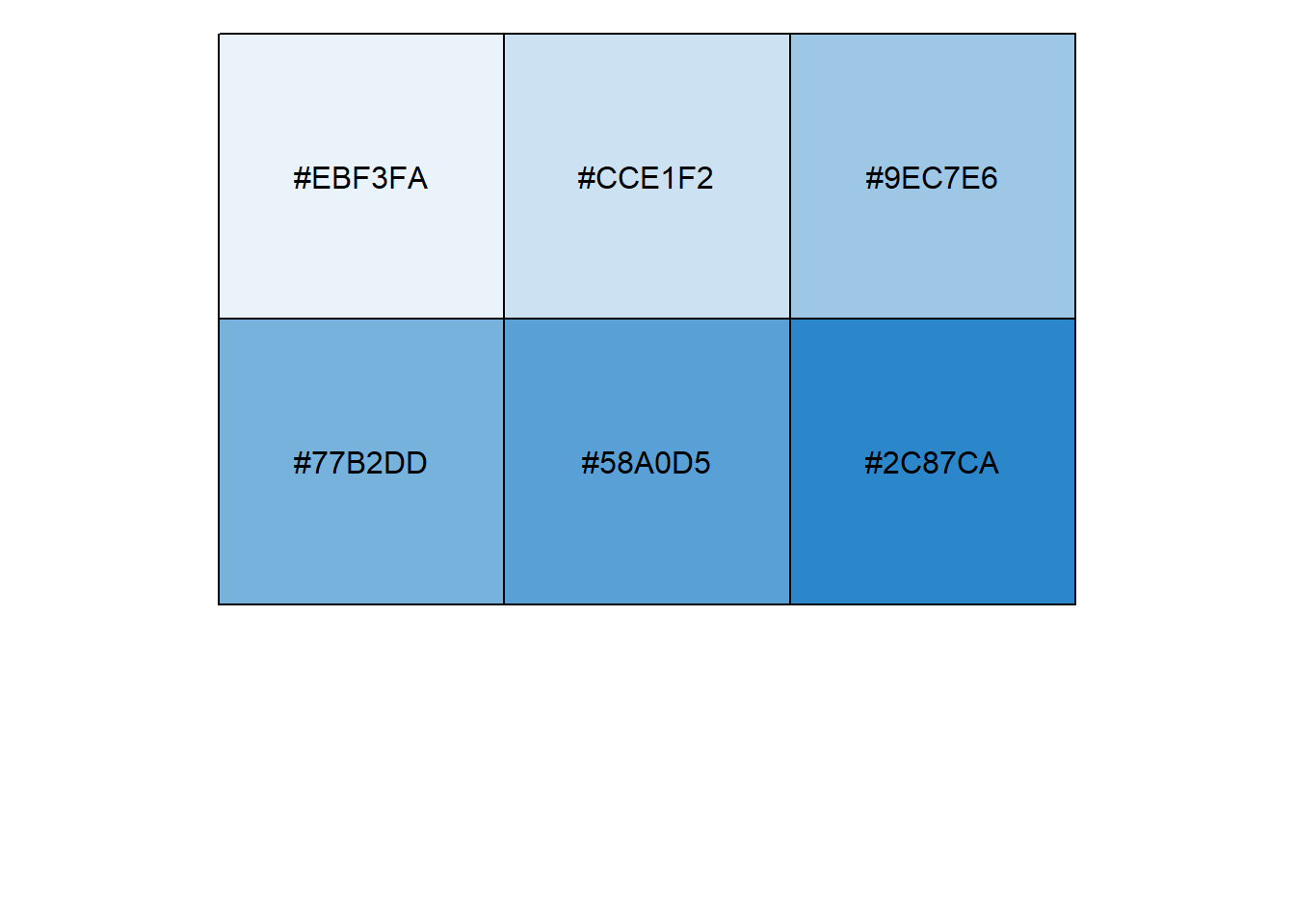
reactable(working_data,
          # Sorting our table based on the FIFA ranking by default
          defaultSorted = "Fifa_rank",
          # Defining vertical and horizontal alignment of each column cell to be center by default
          defaultColDef = colDef(
            vAlign = "center",
            align = "center"
          ),
          columns = list(
          # Embedding country flag images into the first column. You may specify the height and width of the cell.
          ImageURL = colDef(cell = embed_img(working_data,width = 45, height = 40,
                                             horizontal_align = "center"), name = ""),
          Team = colDef(name = "Team",
                          width = 115),
          Fifa_rank = colDef(name = "FIFA Ranking"),
          # Visualising ranking points using bar charts.
          Ranking_points = colDef(name = "FIFA Ranking Points",
                                    defaultSortOrder = "desc",
                                    align = "left",
                                    width = 180,
                                    cell = data_bars(working_data,
                                                     fill_color = "#FEC310",
                                                     bar_height = 10,
                                                     text_position = "outside-base",
                                                     text_size = 15,
                                                     background = "#e1e1e1")),
          Round_16 = colDef(name = "Round of 16",
                            style = function(value){
                              value
                              normalised <- (value-min(working_data$Round_16))/(max(working_data$Round_16)--min(working_data$Round_16))
                              color <- good_color(normalised)
                              list(background = color)}),
          Quarter_finals = colDef(
            name = "Quarter-Final",
            style = function(value){
                              value
                              normalised <- (value-min(working_data$Quarter_finals))/(max(working_data$Quarter_finals)--min(working_data$Quarter_finals))
                              color <- good_color(normalised)
                              list(background = color)}),
          Semi_finals = colDef(
            name = "Semi-Final",
            style = function(value){
                              value
                              normalised <- (value-min(working_data$Semi_finals))/(max(working_data$Semi_finals)--min(working_data$Semi_finals))
                              color <- good_color(normalised)
                              list(background = color)}),
          Finals = colDef(
            name = "Final",
            style = function(value){
                              value
                              normalised <- (value-min(working_data$Finals))/(max(working_data$Finals)--min(working_data$Finals))
                              color <- good_color(normalised)
                              list(background = color)}),
          Wins = colDef(
            name = "Champion",
            style = function(value){
                              value
                              normalised <- (value-min(working_data$Wins))/(max(working_data$Wins)--min(working_data$Wins))
                              color <- good_color(normalised)
                              list(background = color)})
          ))
Adding Title, Subtitle and Caption
Lastly, we may apply the finishing touch to our table by inputting an appropriate title, subtitle and caption to aid the reader to better understand the table. This can easily be done with functions from the {reactablefmtr} package, and you may customise various options such as font colour, font size and font weight.
reactable(working_data,
          # Display the full table in one page
          pagination = FALSE,
          # Sorting our table based on the FIFA ranking by default
          defaultSorted = "Fifa_rank",
          # Defining vertical and horizontal alignment of each column cell to be center by default
          defaultColDef = colDef(
            vAlign = "center",
            align = "center"
          ),
          columns = list(
          # Embedding country flag images into the first column. You may specify the height and width of the cell.
          ImageURL = colDef(cell = embed_img(working_data,width = 45, height = 40,
                                             horizontal_align = "center"), name = ""),
          Team = colDef(name = "Team",
                          width = 115),
          Fifa_rank = colDef(name = "FIFA Ranking"),
          # Visualising ranking points using bar charts.
          Ranking_points = colDef(name = "FIFA Ranking Points",
                                    defaultSortOrder = "desc",
                                    align = "left",
                                    width = 180,
                                    cell = data_bars(working_data,
                                                     fill_color = "#FEC310",
                                                     bar_height = 10,
                                                     text_position = "outside-base",
                                                     text_size = 15,
                                                     background = "#e1e1e1")),
          Round_16 = colDef(name = "Round of 16",
                            style = function(value){
                              value
                              normalised <- (value-min(working_data$Round_16))/(max(working_data$Round_16)--min(working_data$Round_16))
                              color <- good_color(normalised)
                              list(background = color)}),
          Quarter_finals = colDef(
            name = "Quarter-Final",
            style = function(value){
                              value
                              normalised <- (value-min(working_data$Quarter_finals))/(max(working_data$Quarter_finals)--min(working_data$Quarter_finals))
                              color <- good_color(normalised)
                              list(background = color)}),
          Semi_finals = colDef(
            name = "Semi-Final",
            style = function(value){
                              value
                              normalised <- (value-min(working_data$Semi_finals))/(max(working_data$Semi_finals)--min(working_data$Semi_finals))
                              color <- good_color(normalised)
                              list(background = color)}),
          Finals = colDef(
            name = "Final",
            style = function(value){
                              value
                              normalised <- (value-min(working_data$Finals))/(max(working_data$Finals)--min(working_data$Finals))
                              color <- good_color(normalised)
                              list(background = color)}),
          Wins = colDef(
            name = "Champion",
            style = function(value){
                              value
                              normalised <- (value-min(working_data$Wins))/(max(working_data$Wins)--min(working_data$Wins))
                              color <- good_color(normalised)
                              list(background = color)})
          ))|>
  # Add title of table
  add_title("FIFA World Cup 2022",
            font_color = "#1077C3")|>
  # Add subtitle of table
  add_subtitle("History of participating teams in the knockout stages of the World Cup competition",
               font_weight = "normal",
               margin = c(5,0,10,0))|>
  # Add caption of table
  add_source("Note: Data of knockout stages excluded year 1950 competition as the finals were played in a round robin format instead",
             font_style = "italic",
             font_size = 14)|>
  add_source("DATA: KAGGLE| TABLE: TOU NIEN XIANG | NIENXIANGTOU.COM",
             font_color = "#C8C8C8",
             margin = c(5,0,0,0))
FIFA World Cup 2022
History of participating teams in the knockout stages of the World Cup competition
Note: Data of knockout stages excluded year 1950 competition as the finals were played in a round robin format instead
DATA: KAGGLE| TABLE: TOU NIEN XIANG | NIENXIANGTOU.COM
Useful links
I have mainly learned how to create the above table from the useful links below.
Interactive data tables for R - Coding examples on various functions of the {reactable} package by its developer, Greg Lin
Reactable - An Interactive Tables Guide - Blog post by Thomas Mock highlighting how to add and format background colours of the table
Tables don’t have to be necessarily boring, and many packages are available to help us to spice things up. I look forward to explore more functionality of the {reactable} package!
This project is created using R programming language. Full code can be found on my github.